Minimal kernel with Google Colab : An addition
All the exercices of the module are to be done in the Google Colab
environment. So, start by logging you on
the Google Colab
webpage.
Google Colab allows you to write and execute code in an interactive
environment called a Colab notebook. You can write different kind of
codes, including CUDA codes. In order to tell Google Colab that you
want to use a GPU, you have to change the default runtime in the
menu Runtime>Change Runtime Type and set Runtime type
to Python 3 and Hardware accelerator
to GPU.
You will find
here
a notebook in which :
- the first cell corresponds to our CUDA program;
- the second cell compile the cuda program;
- the last one launches the program.
The given program makes an addition on the GPU thanks to a kernel executed by a single thread.
- Read the program.
- Load the code, compile it and launch the program using the buttons "play" on the left of the
code blocks.
Remarks :
- %%writefile line is related to the notebook and store the code
as a file with the given name.
- Do not forget to specify the use of a GPU in Google Colab environment.
Minimal kernel with Error management
CUDA calls on GPU fail with silent error. In
this notebook,
we highlight the value of protecting your CUDA calls to detect
errors :
- In the first section named "Raw code", you can read a CUDA code written
without any precautions. Run the code and observe the result. You
may not be agree with the result of
2 + 2 = 0.
- In the second section, we introduce how
debugging this code with the debugger cuda-gdb.
For this purpose, you need to :
- compile adding the options"-g -G" so that debugging
symbols are included. For this purpose, you need
to save your code in a file by beginning it with "%%writefile
file_name.cu" (instead of "%%cu") and compile it explicitly in a
separate cell. Note that in a notebook, shell commands start
with ! .
- write in a file the sequence of instructions to be followed by
the debugger. Indeed, cuda-gdb is interactive (you are
expected to type commands as you go along), but running
programs in the Colab environnement is not. Typical
commands would go like this:
- set the debugger up to check lots of possible errors:
- memory checks : memcheck on,
- stop in case of API failures : api_failures stop,
- stop on exceptions : catch throw,
- run the program (possibly with command line options) :
r option1 option2 ,
- show the kernel call stack (GPU) : bt,
- print all local variables : info locals,
- switch to the host thread : thread 1
- and show the host program call stack (CPU) : bt.
- call the debugger with your program and execute the
commands from debug_instructions.txt. If your program terminates fine,
cuda-gdb will complain that there is no stack (since the
program finished)
After running all cells of the "Debugging" notebook section, you
should get an exception and lots of information. There is an
illegal address detected in line 5 of add.cu, which is in kernel
add. You may identify and fix the problem by hand but it should have
been caught by the cuda errors management, object of the next section.
Note : If you do use printf to debug, be sure to flush the buffer by
adding a line break at the end. This applies to any C
program. Example: printf("Works up to here\n"); .
Nevertheless, the interface between the Jupyter Notebook and the
executed program is a little fragile. So if your program crashes,
there might not be ANY output at all, even if you have printf
everywhere.
- In the third section "Code with error management", we
instrument the code to check the return error code of calls to
CUDA. The program should fail now (and no longer crash and
give a wrong result).
As CUDA calls on GPU fail with silent error, it is required
to retrieve and check the error code of all of them. Since
kernel calls do not have a return value, first of all, you can check
for invalid launch argument with the error code of
cudaPeekAtLastError(); and then, you can check if errors
occurred during the kernel execution thanks to the error code of
cudaDeviceSynchronize, that forces the kernel completion.
Note that most of the time, a developper will use the cudaMemcpy
as synchronization primitive (the cudaDeviceSynchronize would be
in duplicate then). In this cas, the cudaMemcpy call can return
either errors which occurred during the kernel execution or
those from the memory copy itself.
- In the last section, we have outsourced the error management
code so that you can use it more easily in the rest of your
exercises.
Notice that the first line of the cell has
changed. Now, each cell is saved as a file and the compilation and
execution are launched explicitly in two additional cells with a
shell command. Note that in a notebook, shell commands start
with ! .
- Last but not least, it remains you to fix the problem.
First parallel computation kernel: SAXPY
We implement here the linear application y = ax + y on an
large vector whose CPU code is:
  void saxpy(float *x, float *y, int len, float a){
    for (int i = 0; i < len; ++i)
      y[i] = a*x[i] + y[i];
  }
- Open a new notebook whose starting point can
be this
one.
- First of all, set up the error management.
- Complete the program to
- copy data to the GPU memory,
- implement a calculation kernel, which you call
saxpy,
which processes one element x of an array passed as a parameter,
the processed element being identified from the
current thread identifiers,
- run the calculation kernel
saxpy in order to treat
all elements of the vector,
- copy the result from the GPU memory to memory
of the host,
- display the first 10 and last 10 results for verification.
- After you have modified your program to set the
vector size, experiment your program with an vector of
10.000 elements and 100.000 elements.
- Test several combinations of "number of blocks" / "number of
threads per block", for arrays of different sizes and
observe the performance achieved.
- Compare them also to those
obtained using a CPU thanks to timers.
Warning! Launch your experiments within the same program.
so that the different tests can be performed on the same hardware.
and are therefore comparable.
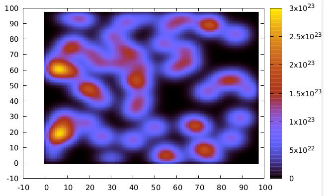
Convolution
The convolution application calculates a 2D diffusion (type of the heat
equation). A matrix contains values (e.g. the temperature of a
point in space), and at each iteration a 5-point stencil is applied:
for each point (i,j), one calculates :
.
The program in this notebook generates a random number of "hot spots", calculates
several iterations and writes the result to the result.dat file.
This result can be visualized with the plot.gp
script (which requires GNUplot software).
- Write the kernel to run the calculation on the GPU.
- We have not had much opportunity yet to discuss the different
types of memory available on a GPU as this will be the subject of
next week course. However, be aware that there is a small memory to
store constant data.
Place the convolution weight mask in this constant memory by
declaring it in this way :
__constant__ double D_WEIGHT[3][3];
and initiliaze it with a transfer :
cudaMemcpyToSymbol(D_WEIGHT, weight, 3*3*sizeof(double));
- Compare the performances.
- We could do even better using shared memory but we are saving that for next week.
Congrats! You have reached the end of the session! See you next week to tackle the optimization of the basic operation of deep learning, the multiplication of matrices!
Square Matrix Multiplication
Here you have to implement the multiplication of square matrices C = A x B.
- In
this
notebook, you will find a code skeleton that will allow you to
implement and compare the different matrix multiplication strategies.
- Basic version : Taking the previous notebook as a starting point,
implement a version that does use the global memory of the
GPU. Each block being limited to 1024 threads, a square tile has
maximum dimensions of 32x32. Multiply on matrices of slightly
larger dimensions. (e.g., let work 20 blocks in parallel),
with a 32x32 tiling.
- Tiled version :
By following the explanations given in the course,
implement into the same notebook the tiled version.
- Compare the execution times of the two implementations. Also
compare the execution time by varying the tile size (eg when TILE_WIDTH=16 and
TILE_WIDTH=32). Note: In order to obtain
stable performance, run the computation several times and consider the
average execution time for your comparisons.