
In fact, the compiler generally manages to generate a binary which exploits all the capacities of the processor. But the compiler sometimes fails and generates non-optimized code. We must therefore be able to detect the problem, and be able to write code that the compiler can optimize.
1965 - 2005
\(\implies\) Increased processor performance
Since 2005
Source: https://github.com/karlrupp/microprocessor-trend-data
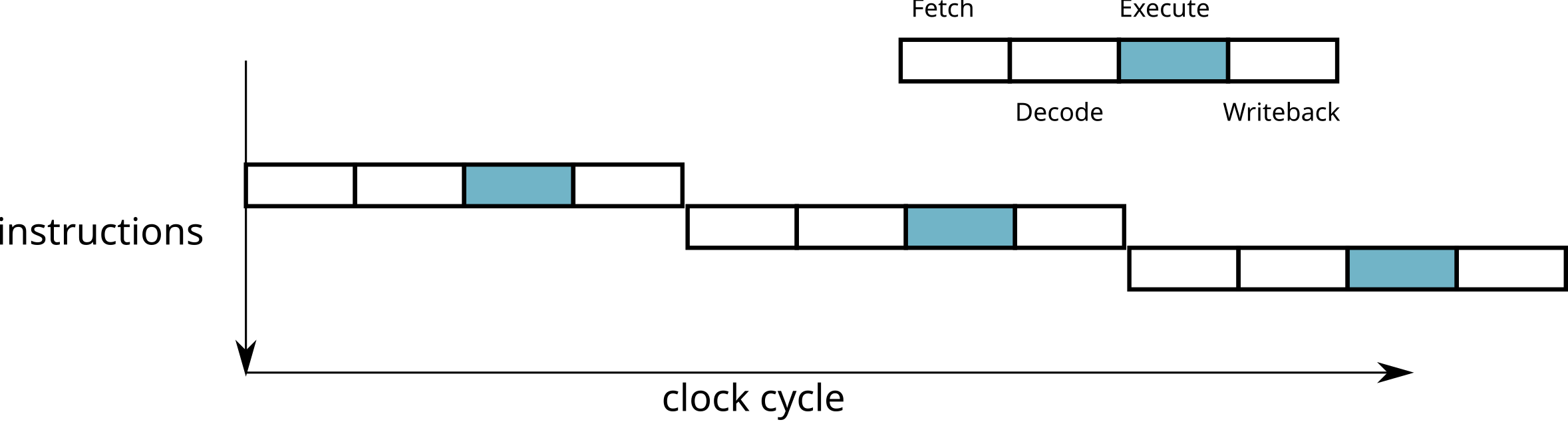
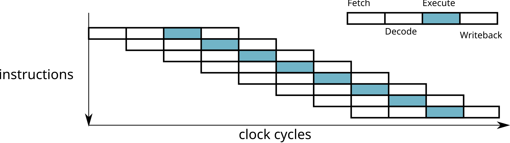
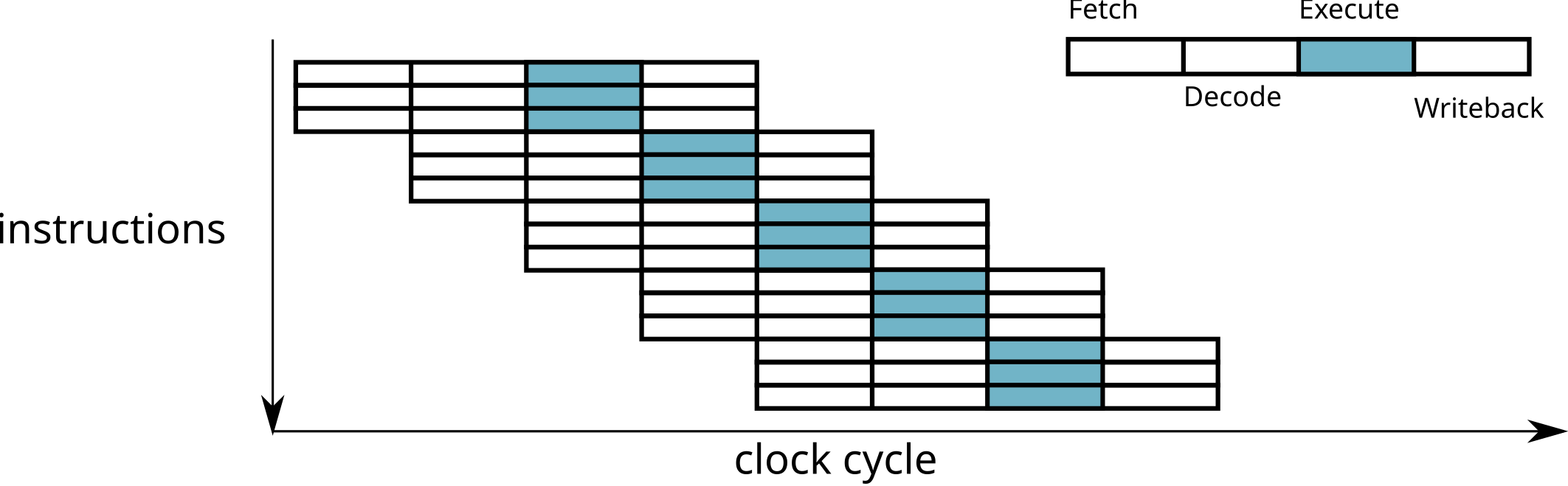
The number of steps required to execute an instruction depends on the processor type (Pentium 4: 31 steps, Intel Haswell: 14-19 steps, ARM9: 5 steps, etc.)
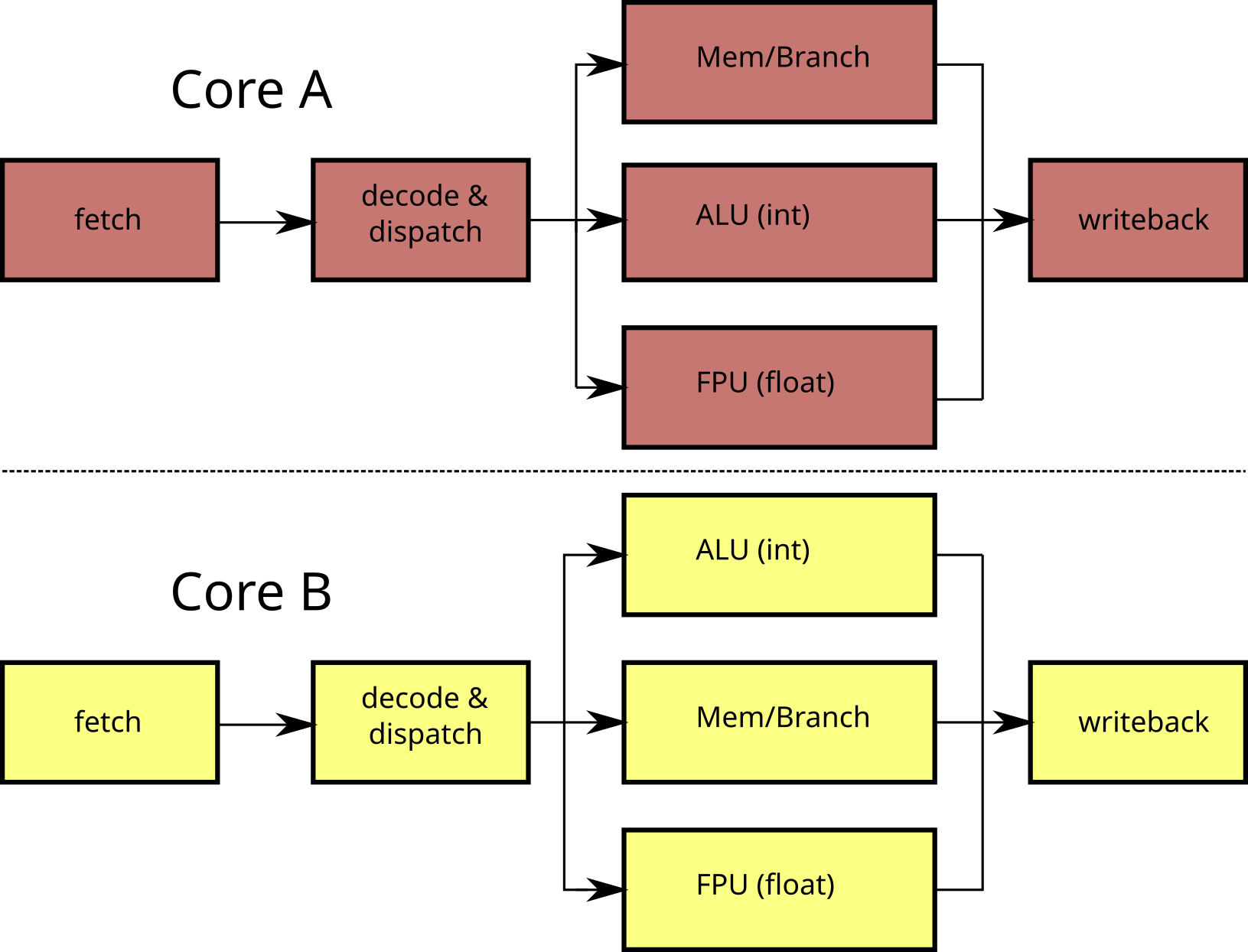
At each stage, several circuits are used
\(\rightarrow\) One instruction is executed at each cycle
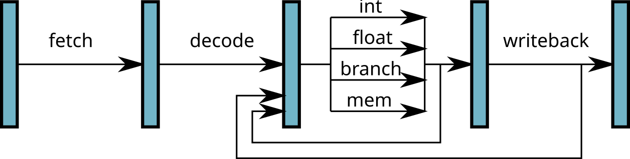
\(\implies\) several instructions executed simultaneously!
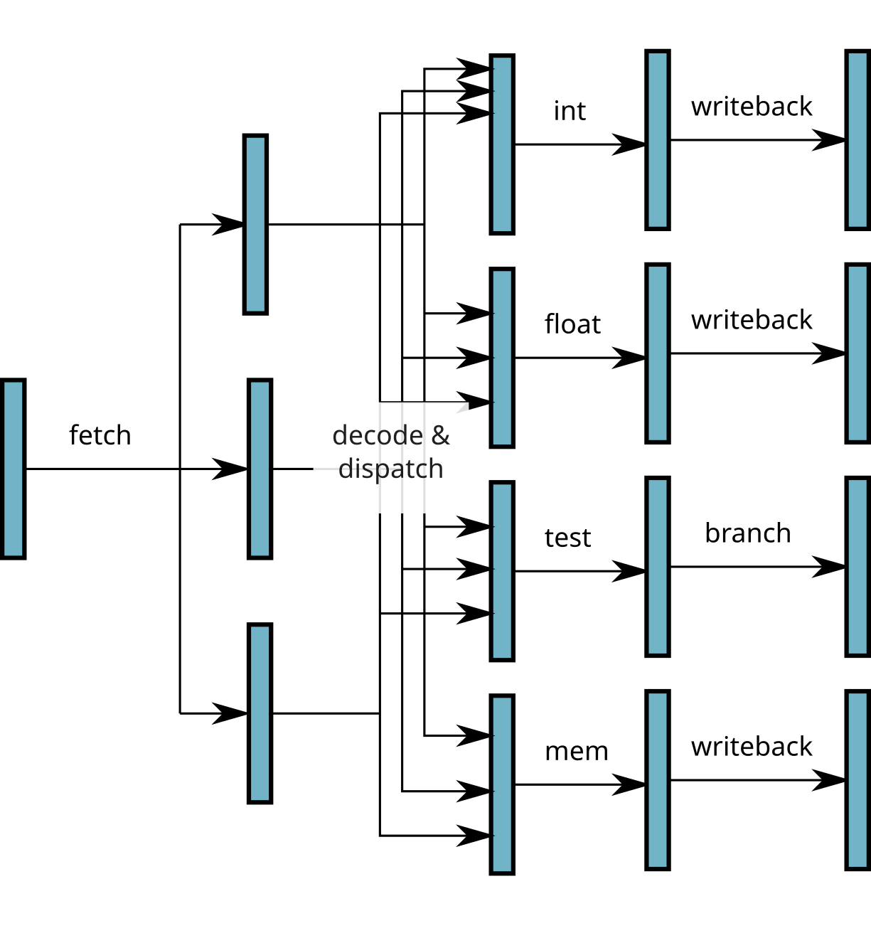
Limitations of the superscalar:
There should be no dependency between statements executed simultaneously.
Example of non-parallelizable instructions
a = b * c;
d = a + 1;
    cmp a, 7    ; a > 7 ?
    ble L1
    mov c, b    ; b = c
    br L2
L1: mov d, b    ; b = d
L2: ...\(\implies\) waste of time
The cost of a wrong choice when loading a branch depends on pipeline depth: the longer the pipeline, the longer it takes to empty it (and therefore wait before executing an instruction). For this reason (among others), the depth of the pipeline in a processor is limited.
0x12 loop:
         ...
0x50     inc eax
0x54     cmpl eax, 10000
0x5A     jl loop
0x5C end_loop:
         ...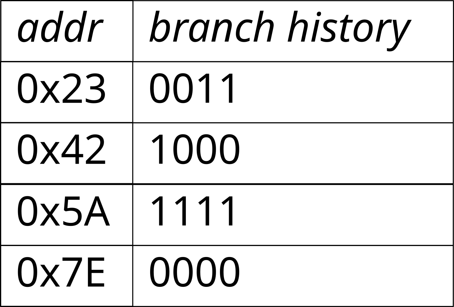
The branch prediction algorithms implemented in modern processors are very advanced and reach a efficiency greater than 98 % (on the SPEC89 benchmark suite).
To know the number of good / bad predictions, we can analyze the
hardware counters of the processor. With the PAPI library <http://icl.cs.utk.edu/projects/papi/>,
the PAPI_BR_PRC and PAPI_BR_MSP counters give
the number of conditional jumps correctly and incorrectly predicted.
Linux perf also allows collects this information (among
others). For example:
$ perf stat -e branches,branch-misses ./branch_prediction  0
is random is not set
100000000 iterations in 1178.597000 ms
result=199999996

 Performance counter stats for './branch_prediction 0':

      2447232697      branches
         6826229      branch-misses            #    0,28% of all branches

       1,179914189 seconds time elapsed

       1,179784000 seconds user
0,000000000 seconds sysfor(i=0; i<size; i++) {
C[i] = A[i] * B[i];
}Example: image processing, scientific computing
Using vector instructions (MMX, SSE, AVX, …)
Instructions specific to a processor type
Process the same operation on multiple data at once
for(i=0; i<size; i+= 8) {
   *pC = _mm_mul_ps(*pA, *pB);
   pA++; pB++; pC++;
}
Vector instructions were democratized at the end of the years 1990 with the MMX (Intel) and 3DNow! (AMD) instruction sets that allow to work on 64 bits (for example to process 2 32-bit operations at once). Since then, each generation of x86 processors brings new extension to the instruction set: SSE2, SSSE3 (128 bit), SSE4, AVX, AVX2 (256 bit), AVX512 (512 bit). The other types of processors also provide vector instructions sets (eg NEON [128 bits], Scalable Vector Extension [SVE] on ARM), or the Vector Extension of RISC-V.
Vector instruction sets are specific to certain processors. The
/proc/cpuinfo file contains (among others) the instructions
sets that are available on the processor of a machine. For example, on
an Intel Core i7:
$ cat  /proc/cpuinfo
processor   : 0
vendor_id   : GenuineIntel
cpu family  : 6
model       : 69
model name  : Intel(R) Core(TM) i7-4600U CPU @ 2.10GHz
stepping    : 1
microcode   : 0x1d
cpu MHz     : 1484.683
cache size  : 4096 KB
physical id : 0
siblings    : 4
core id     : 0
cpu cores   : 2
apicid      : 0
initial apicid  : 0
fpu     : yes
fpu_exception   : yes
cpuid level : 13
wp      : yes
flags : fpu vme de pse tsc msr pae mce cx8 apic sep mtrr pge mca cmov
 pat pse36 clflush dts acpi mmx fxsr sse sse2 ss ht tm pbe syscall nx
 pdpe1gb rdtscp lm constant_tsc arch_perfmon pebs bts rep_good nopl
 xtopology nonstop_tsc aperfmperf eagerfpu pni pclmulqdq dtes64
 monitor ds_cpl vmx smx est tm2 ssse3 sdbg fma cx16 xtpr pdcm pcid
 sse4_1 sse4_2 x2apic movbe popcnt tsc_deadline_timer aes xsave avx
 f16c rdrand lahf_lm abm ida arat epb pln pts dtherm tpr_shadow vnmi
 flexpriority ept vpid fsgsbase tsc_adjust bmi1 avx2 smep bmi2 erms
 invpcid xsaveopt
bugs        :
bogomips    : 5387.82
clflush size    : 64
cache_alignment : 64
address sizes   : 39 bits physical, 48 bits virtual
power management:
[...]
The flags field contains the list of all the
capabilities of the processor, especially the available
instructions sets:
mmx, sse, sse2, ssse3, sse4_1, sse4_2, avx2.
Vector instruction can be used directly in assembler or by exploiting
the intrinsics provided by compilers. However, because of the
number of available instruction sets and since each new processor
generation provides new instructions sets, it is recommended to leave
the compiler optimize the code, for example using the -O3
option.
Problem with superscalar / vector processors:
Simultaneous Multi-Threading (SMT, or Hyperthreading)
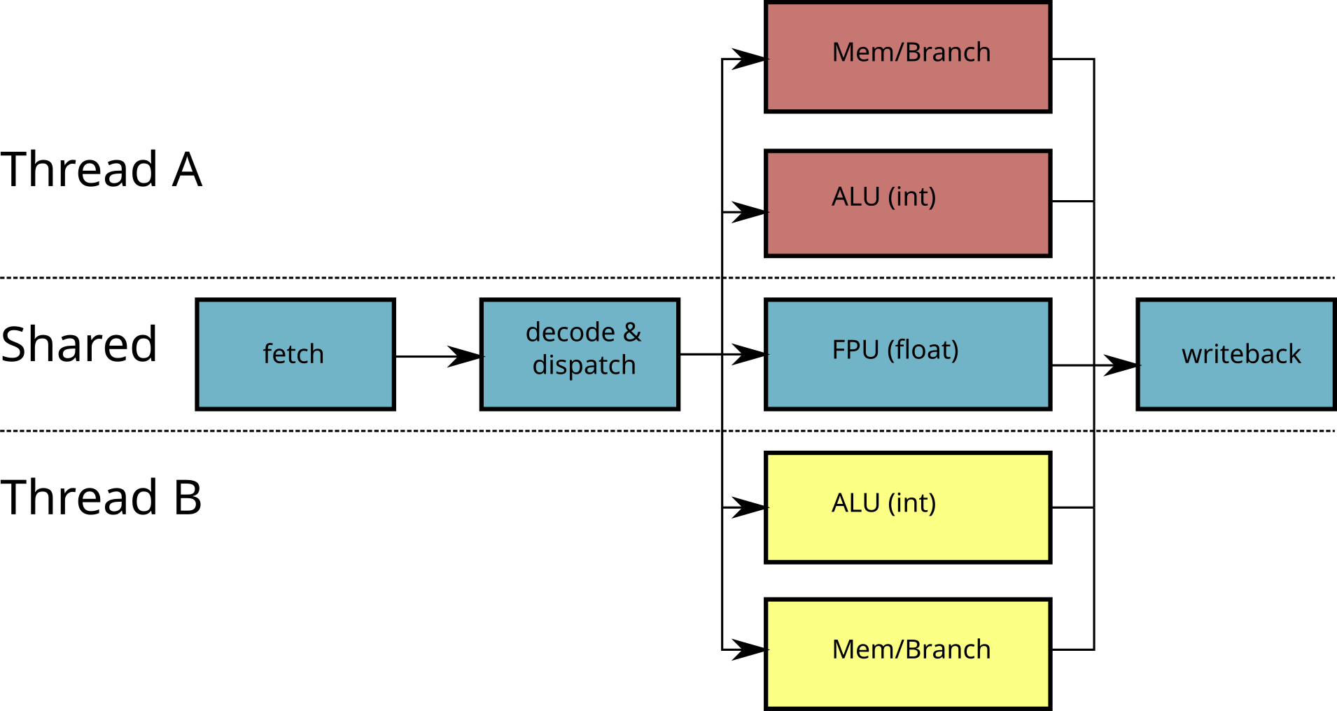
SMT is an inexpensive way to increase the performance of a processor: by duplicating the “small” circuits (ALU, registers, etc.) and by pooling the “big” circuits (FPU, prediction of branches, caches), we can execute several threads simultaneously. The additional cost in terms of manufacturing is light and the gain in performance can be significant.
Since the dispatcher schedules the instructions of several threads, a branch miss-prediction becomes less serious since while the pipeline of the thread is emptied, another thread can be scheduled.
The performance gain when multiple threads are running is not systematic since some circuits remain shared (by example, the FPU).
Limited scalability of SMT
dispatcher is shared
FPU is shared
\(\rightarrow\) Duplicate all the circuits
It is of course possible to combine multi-core with SMT. Most semiconductor foundries produce multi-core SMT processors: Intel Core i7 (4 cores x 2 threads), SPARC T3 Niagara-3 (16 cores x 8 threads), IBM POWER 7 (8 cores x 4 threads).
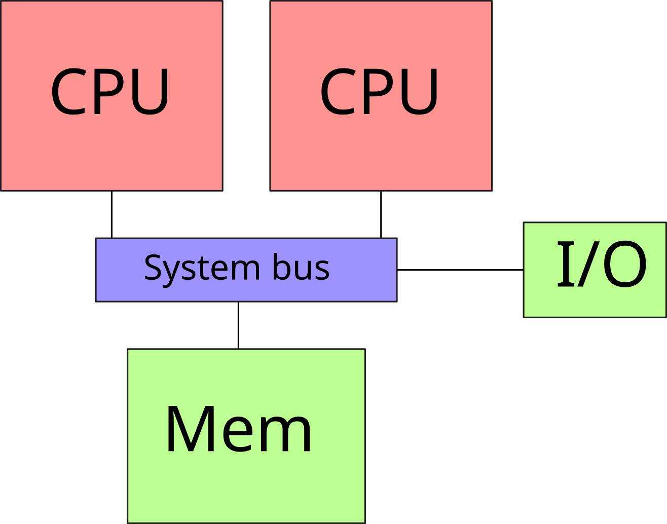
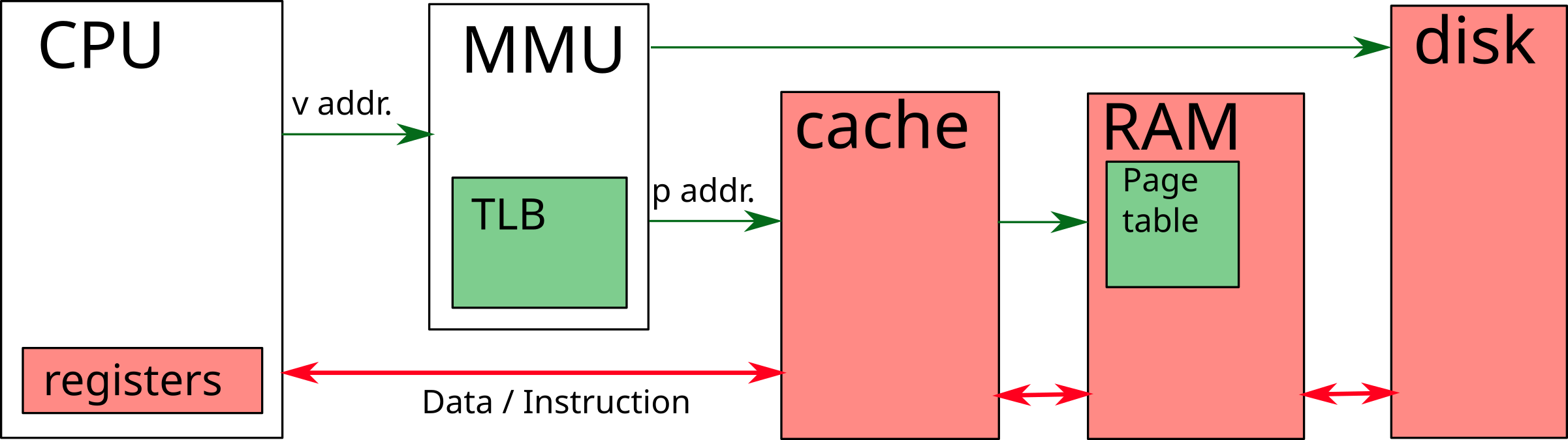
\(\rightarrow\) Non-Uniform Memory Architecture
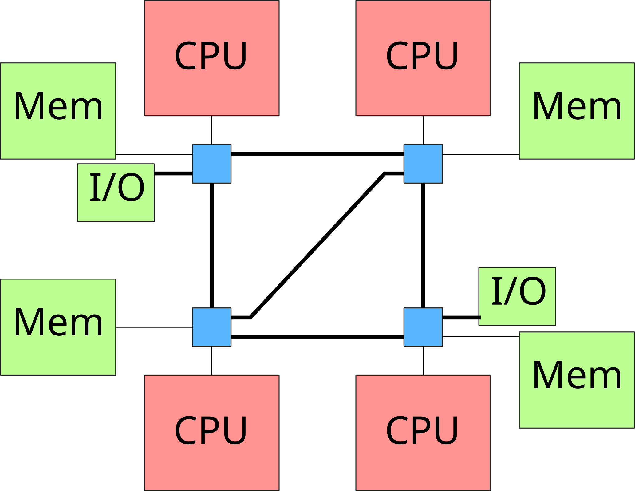
The first NUMA machines (in the 1990s) were simply sets of machines linked by a proprietary network responsible for managing memory transfers. Since 2003, some motherboards allow to plug several Opteron processors (AMD) connected with a HyperTransport link. Intel subsequently developed a similar technology (Quick Path Interconnect, QPI) to connect its Nehalem processors (released in 2007).
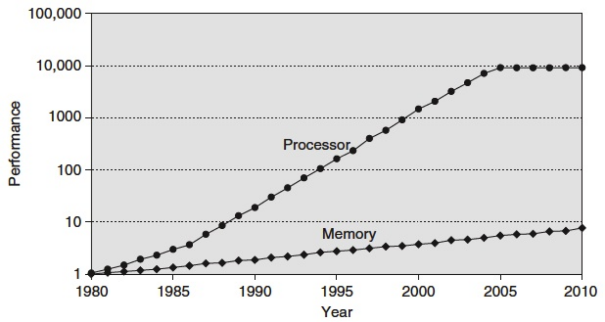
Until the 1990s, performance was limited by the performance of the processor. From the software point of view, developers had to minimize the number of instructions to be executed in order to achieve the best performance.
As the performance of processors increases, the bottleneck is now the memory. On the software side, we therefore seek to minimize the number of costly memory accesses. This pressure on memory is exacerbated by the development of multi-core processors.
For example, an Intel Core i7 processor can generate up to 2 memory access per clock cycle. A 18-core processor with hyper-threading (ie 36 threads) running at 3.1 Ghz can therefore generate \(2 \times 36 \times 3.1 \times 10 ^ 9 = 223.2\) billion memory references per second. If we consider access to 64-bit data, this represents 1662 GiB/s (1.623 TiB/s). In addition to these data accesses, the memory access to the instructions (up to 128 bits per instruction) also have to be taken into account. We thus arrive to a 3325 GiB/s (therefore 3.248 TiB/s !) maximum flow.
For comparison, in 2023 a DDR5 RAM DIMM has a maximum throughput of around 70 GiB/s. It is therefore necessary to set up mechanisms to prevent the processor from spending all its time waiting for memory.
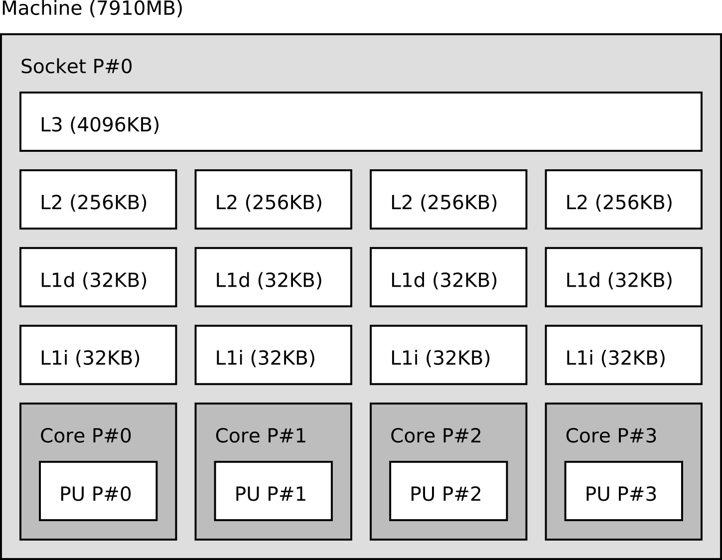
To visualize the memory hierarchy of a machine, you can use the
lstopo tool provided by the hwloc project.
\(\rightarrow\) Mainly used for small caches (ex: TLB)
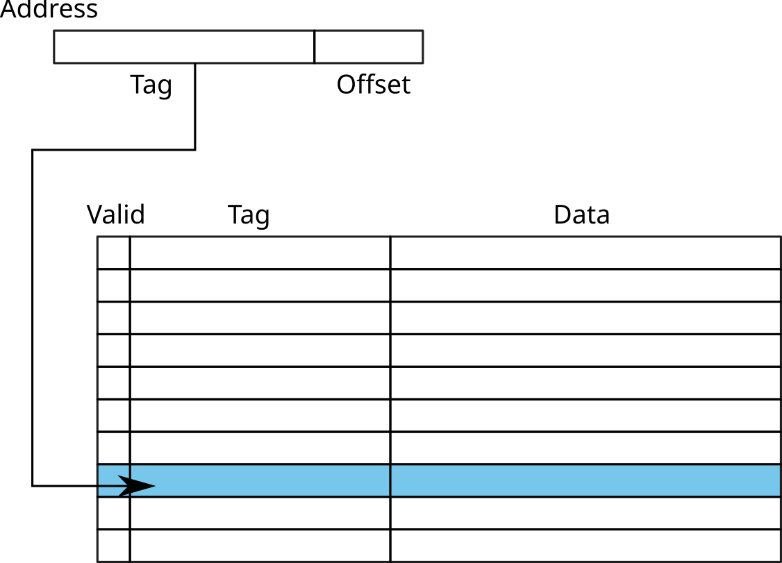
The size of a cache line depends on the processor (usually between 32
and 128 bytes). You can find this information in
/proc/cpuinfo:
$ cat /proc/cpuinfo  |grep cache_alignment
cache_alignment : 64\(\rightarrow\) Direct access to the cache line
Warning: risk of collision
example:
0x12345678 and
0xbff72678
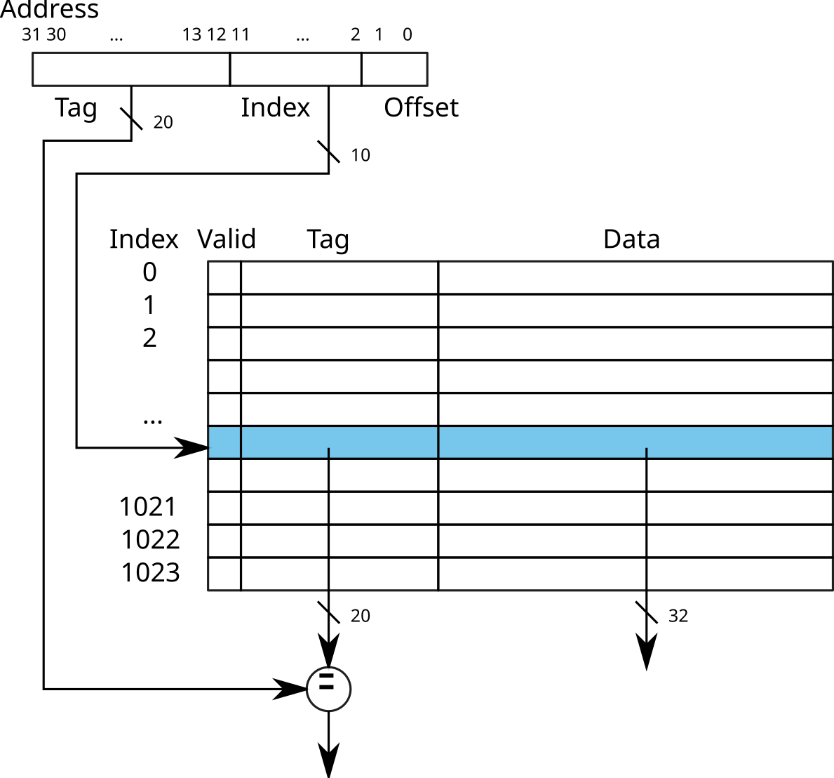
\(\rightarrow\) K-way associative cache (in French: Cache associatif K-voies)
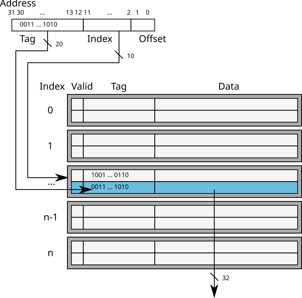
Nowadays, caches (L1, L2 and L3) are generally associative to 4 (ARM Cortex A9 for example), 8 (Intel Sandy Bridge), or even 16 (AMD Opteron Magny-Cours) ways.
What if 2 threads access the same cache line?
Concurrent read: replication in local caches
Concurrent write: need to invalidate data in other caches
Cache snooping: the cache sends a message that invalidates the others caches
To detail this course a little more, we recommend this page web: Modern microprocessors – A 90 minutes guide! http://www.lighterra.com/papers/modernmicroprocessors/.
For (many) more details, read the books [bryant] and [patterson2013computer] which describe in detail the architecture of computers. If you are looking for specific details, read [patterson2011computer].
[bryant] Bryant, Randal E., and David Richard O’Hallaron. “Computer systems: a programmer’s perspective”. Prentice Hall, 2011.
[patterson2013] Patterson, David A and Hennessy, John L. “Computer organization and design: the hardware/software interface”. Newnes, 2013.
[patterson2011] Patterson, David A. “Computer architecture: a quantitative approach”. Elsevier, 2011.